Gallery

A picture is worth atleast 10 lines of code. Here we present images which help illustrate the capabilities, structure, or intention of Pyatoa. Short captions help explain what each image represents.

Waveform Breakdown

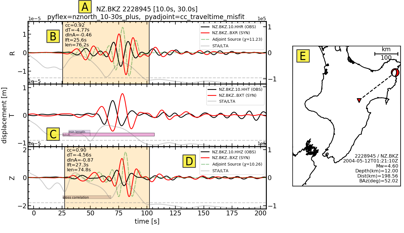
A breakdown of the components of a Pyatoa waveform figure

Misfit assessment for one source-receiver pair, generated using Pyatoa.

1. Waveform title with relevant information like processing parameters.
1. Time windows shown with measurement information.
1. Rejected time windows are shown as color-coded bars.
1. Legend provides component identification and total calculated misfit
1. Source-receiver map

Inspector Gallery

The following figures can be generated by the Inspector class, which facilitates analysis of inversion results generated using SeisFlows.

from pyatoa.scripts.load_example_data import load_example_inspector

insp = load_example_inspector()

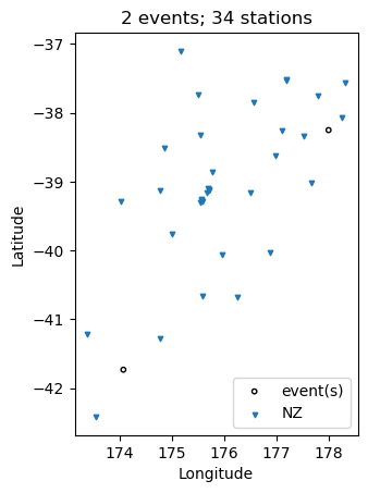
Source-Receiver Metadata

A very simple source-receiver scatter plot can be created with the map function

insp.map(show=True, save=False)

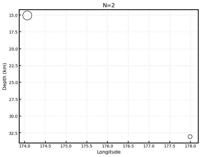
The event_depths functions plots a 2D cross section of all events at depth

insp.event_depths(xaxis="longitude", show=True, save=False)

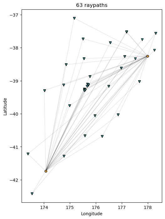
The raypaths function shows connecting lines for any source-receiver pair that has atleast one measurement

insp.raypaths(iteration="i01", step_count="s00", show=True, save=False)

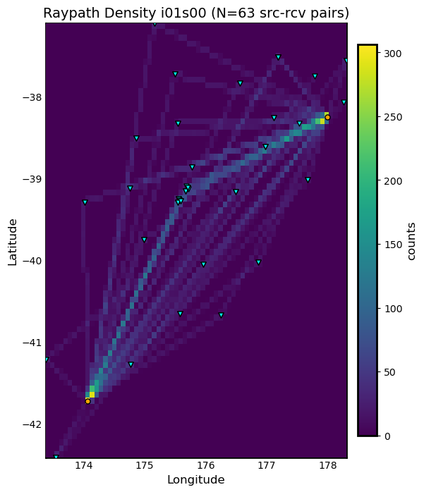
The raypath_density function provides a more detailed raypath plot, which is colored by the density of overlapping raypaths

insp.raypath_density(iteration="i01", step_count="s00", show=True, save=False)

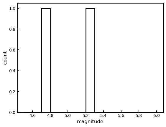
The event_hist function creates a simple event histogram based on event information such as magnitude.

insp.event_hist(choice="magnitude", show=True, save=False)

Misfit Window Timing

The following plotting functions are concerned with visualizing the time dependent part of the measurements

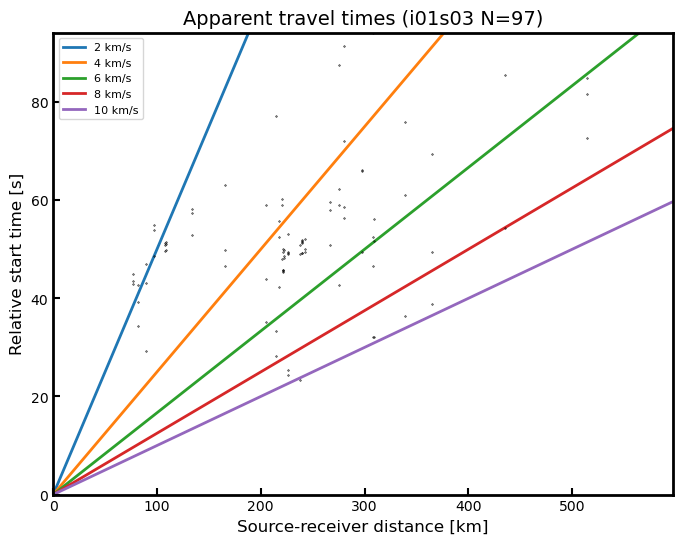
The travel_times function plots a proxy for phase arrivals, similar to a seismic record section.

insp.travel_times(t_offset=-20, constants=[2, 4, 6, 8, 10], show=True, save=False)

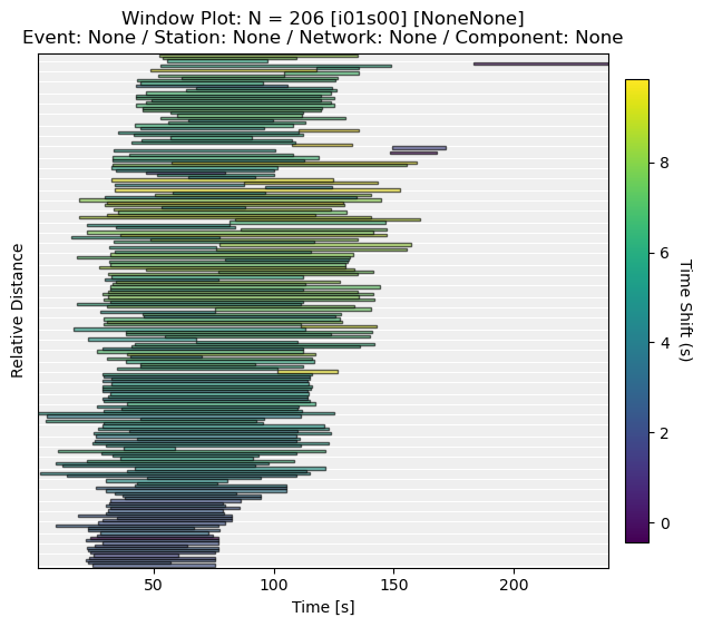
The plot_windows function plots time windows (as bars) against source receiver distance, illustrating seismic phases included in the inversion.

insp.plot_windows(iteration="i01", step_count="s00", show=True, save=False)

Inversion Statistics

The following plotting functions help the user understand how an inversion is progressing by comparing iterations against one another. These are common inversion statistics plots shown in many tomography publications.

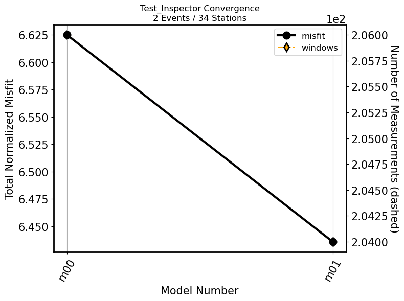
The convergence function plots total misfit per iteration over the course of an inversion. An additional Y axis is used to plot the number of windows for each iteration (or the overall length of the time windows)

insp.convergence(windows="nwin", show=True, save=False)

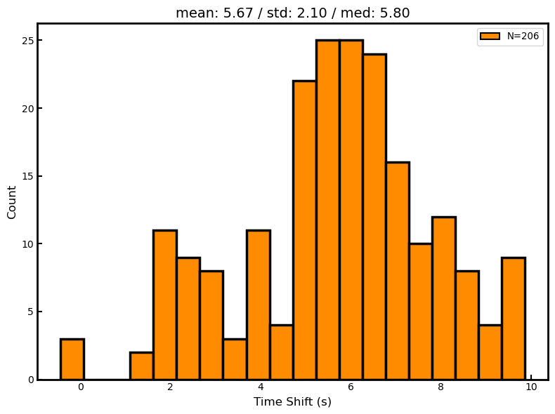
The hist function generates histograms for a given measurement column, such as overall cross correlation or amplitude anomaly.

insp.hist(iteration="i01", step_count="s00", choice="cc_shift_in_seconds", show=True, save=False)

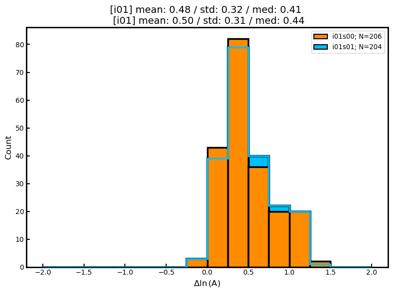
The hist function can also be used to generate two sets of histograms that compare one iteration to another:

insp.hist(iteration="i01", step_count="s00",
          iteration_comp="i01", step_count_comp="s01",
          choice="dlnA", show=True, save=False)

Measurement Statistics

These plotting functions allow the user to plot measurements for a given evaluation in order to better understand the statistical distribution of measurements, or comparisons against one another.

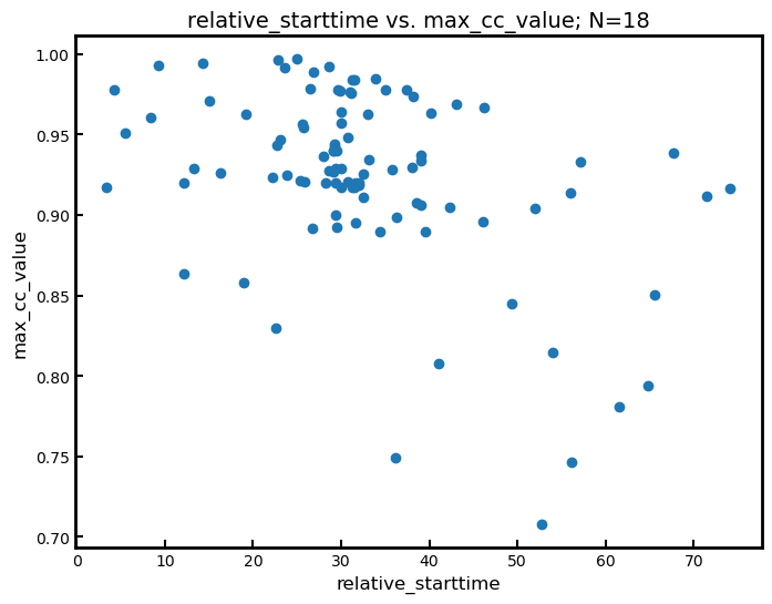
The scatter function compares any two attributes in the windows dataframe

insp.scatter(x="relative_starttime", y="max_cc_value", show=True, save=False)

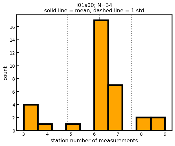
The measurement_hist function generates histograms of source or receiver metadata. Useful for identifying events or stations which may be outliers in terms of overall measurements.

insp.measurement_hist(iteration="i01", step_count="s00", choice="station", show=True, save=False)

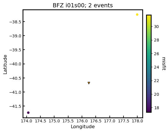
The station_event_misfit_map creates a map for a single station. All other points correspond to events which the station has recorded. Colors of these markers correspond to given measurement criteria.

insp.station_event_misfit_map(station="BFZ", iteration="i01", step_count="s00",
                              choice="misfit", show=True, save=False)

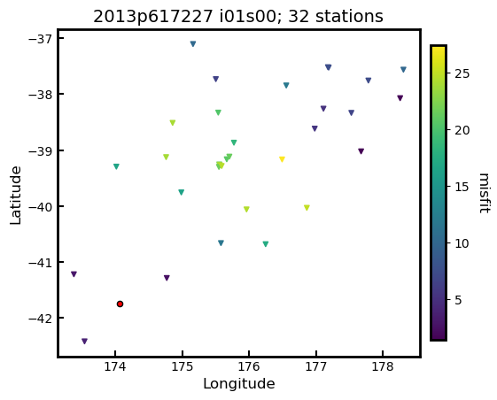
The station_event_misfit_map creates a map for a single event. All other points correspond to stations which have recorded the event. Colors of these markers correspond to given measurement criteria.

insp.event_station_misfit_map(event="2013p617227", iteration="i01",
                              step_count="s00", choice="misfit",
                              show=True, save=False)

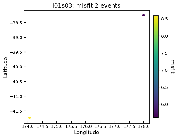
The event_misfit_map plots all events on a map and their corresponding scaled misfit value for a given evaluation (defaults to last evaluation in the Inspector).

insp.event_misfit_map(choice="misfit", show=True, save=False)